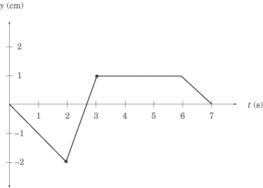
Any point on this graph gives us the position of the ant at a particular moment
in time. For instance, the point at (2,–2)
tells us that, two seconds after it started moving, the ant was two centimeters
to the left of its starting position, and the point at
(3,1) tells us that, three seconds after it
started moving, the ant is one centimeter to the right of its starting position.
Let’s read what the graph can tell us about the ant’s movements. For the first
two seconds, the ant is moving to the left. Then, in the next second, it
reverses its direction and moves quickly to y
= 1. The ant then stays still at y =
1 for three seconds before it turns left again and moves back to where it
started. Note how concisely the graph displays all this information.
Calculating Velocity
We know the ant’s displacement, and we know how long it takes to move from place
to place. Armed with this information, we should also be able to determine the
ant’s velocity, since velocity measures the rate of change of displacement over
time. If displacement is given here by the vector
y, then the velocity of the ant is

If you recall, the slope of a graph is a measure of rise over run; that is, the
amount of change in the y direction divided by the amount of change in
the x direction. In our graph,
?y
is the change in the y direction and
?t
is the change in the x direction, so
div>
is a measure of the slope of the graph. For any position vs.
time graph, the velocity at time t is equal to the slope of the line at
t. In a graph made up of straight lines, like the one above, we can
easily calculate the slope at each point on the graph, and hence know the
instantaneous velocity at any given time.
We can tell that the ant has a velocity of zero from
t = 3 to
t = 6, because the slope of the line
at these points is zero. We can also tell that the ant is cruising along at the
fastest speed between t = 2 and
t = 3, because the position vs. time
graph is steepest between these points. Calculating the ant’s average velocity
during this time interval is a simple matter of dividing rise by run, as we’ve
learned in math class.

Average Speed
Although the total displacement in the first three seconds is one centimeter to
the right, the total distance traveled is two centimeters to the left, and then
three centimeters to the right, for a grand total of five centimeters. Thus, the
average speed is not the same as the average velocity of the ant. Once we’ve
calculated the total distance traveled by the ant, though, calculating its
average speed is not difficult:
5cm/3s=1.67cm/s
Curved Position vs. Time Graphs
This is all well and good, but how do you calculate the velocity of a curved
position vs. time graph? Well, the bad news is that you’d need calculus. The
good news is that subject test Physics doesn’t expect you to use calculus, so if you
are given a curved position vs. time graph, you will only be asked qualitative
questions and won’t be expected to make any calculations. A few points on the
graph will probably be labeled, and you will have to identify which point has
the greatest or least velocity. Remember, the point with the greatest slope has
the greatest velocity, and the point with the least slope has the least
velocity. The turning points of the graph, the tops of the “hills” and the
bottoms of the “valleys” where the slope is zero, have zero velocity.
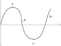
In this graph, for example, the velocity is zero at points A and C,
greatest at point D, and smallest at point B. The velocity at point B
is smallest because the slope at that point is negative. Because velocity
is a vector quantity, the velocity at B would be a large negative number.
However, the speed at B is greater even than the speed at D: speed is a scalar
quantity, and so it is always positive. The slope at B is even steeper than
at D, so the speed is greatest at B.
Velocity vs. Time Graphs
Velocity vs. time graphs are the most eloquent kind of graph we’ll be looking at
here. They tell us very directly what the velocity of an object is at any given
time, and they provide subtle means for determining both the position and
acceleration of the same object over time. The “object” whose velocity is
graphed below is our ever-industrious ant, a little later in the day.
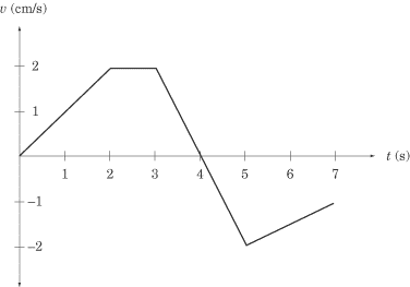
We can learn two things about the ant’s velocity by a quick glance at the graph.
First, we can tell exactly how fast it is going at any given time. For instance,
we can see that, two seconds after it started to move, the ant is moving at 2 cm/s. Second,
we can tell in which direction the ant is moving. From t = 0 to t = 4, the velocity is positive,
meaning that the ant is moving to the right. From t = 4 to t = 7, the velocity is negative,
meaning that the ant is moving to the left.
Calculating Acceleration
We can calculate acceleration on a velocity vs. time graph in the same way that
we calculate velocity on a position vs. time graph. Acceleration is the rate of
change of the velocity vector,?v/?t, which expresses itself as the slope of the
velocity vs.
time graph. For a velocity vs. time graph, the acceleration at time t is equal to
the slope of the line at t.
What is the acceleration of our ant at t = 2.5 and t = 4? Looking quickly at the graph,
we see that the slope of the line at t = 2.5 is zero and hence the acceleration is
likewise zero. The slope of the graph between t = 3 and t = 5 is constant, so we can
calculate the acceleration at t = 4 by calculating the average acceleration between
t = 3 and t = 5:
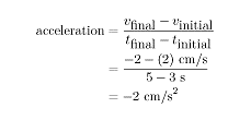
The minus sign tells us that acceleration is in the leftward direction,
since we’ve defined the y-coordinates in such a way that right is positive
and left is negative. At t = 3, the ant is moving to the right at 2 cm/s,
so a leftward acceleration means that the ant begins to slow down. Looking
at the graph, we can see that the ant comes to a stop at t = 4, and then
begins accelerating to the right.
Calculating Displacement
Velocity vs. time graphs can also tell us about an object’s displacement.
Because velocity is a measure of displacement over time, we can infer that:
displacement = velocity × time
Graphically, this means that the displacement in a given time interval
is equal to the area under the graph during that same time interval.
If the graph is above the t-axis, then the positive displacement is
the area between the graph and the t-axis. If the graph is below the t-axis,
then the displacement is negative, and is the area between the graph and the
t-axis. Let’s look at two examples to make this rule clearer.
First, what is the ant’s displacement between t = 2 and t = 3?
Because the velocity is constant during this time interval,
the area between the graph and the t-axis is a rectangle of width 1 and height 2.

The displacement between t = 2 and t = 3 is the
area of this rectangle, which is 1 cm/s × 2s = 2 cm to the right.
Next, consider the ant’s displacement between t = 3 and t = 5.
This portion of the graph gives us two triangles, one above the
t-axis and one below the t-axis.

Both triangles have an area of 1 /2(1 s)(2 cm/s) = 1 cm. However,
the first triangle is above the t-axis, meaning that displacement is
positive, and hence to the right, while the second triangle is below
the t-axis, meaning that displacement is negative, and hence to the
left. The total displacement between t = 3 and t = 5 is:
1cm- 1cm=0
In other words, at t = 5, the ant is in the same place as it was at t = 3.
Curved Velocity vs. Time Graphs
As with position vs. time graphs, velocity vs. time graphs may also be curved.
Remember that regions with a steep slope indicate rapid acceleration or deceleration,
regions with a gentle slope indicate small acceleration or deceleration, and the turning
points have zero acceleration.
Acceleration vs. Time Graphs
After looking at position vs. time graphs and velocity vs. time graphs,
acceleration vs. time graphs should not be threatening. Let’s look at the acceleration
of our ant at another point in its dizzy day.

Acceleration vs. time graphs give us information about acceleration
and about velocity. subject test Physics generally sticks to problems that
involve a constant acceleration. In this graph, the ant is accelerating
at 1 m/s2 from t = 2 to t = 5 and is not accelerating between t = 6
and t = 7; that is, between t = 6 and t = 7 the ant’s velocity is constant.
Calculating Change in Velocity
Acceleration vs. time graphs tell us about an object’s velocity in the same
way that velocity vs. time graphs tell us about an object’s displacement.
The change in velocity in a given time interval is equal to the area under
the graph during that same time interval. Be careful: the area between the
graph and the t-axis gives the change in velocity, not the final velocity or
average velocity over a given time period.
What is the ant’s change in velocity between t = 2 and t = 5? Because
the acceleration is constant during this time interval, the area between
the graph and the t-axis is a rectangle of height 1 and length 3.

The area of the shaded region, and consequently the change in velocity
during this time interval, is 1 cm/s2 · 3 s = 3 cm/s to the right. This doesn’t
mean that the velocity at t = 5 is 3 cm/s; it simply means that the velocity is 3 cm/s
greater than it was at t = 2. Since we have not been given the velocity at t = 2, we can’t
immediately say what the velocity is at t = 5.
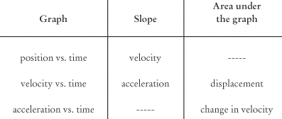
Summary of Rules for Reading Graphs
You may have trouble recalling when to look for the slope and when to look for
the area under the graph. Here are a couple handy rules of thumb:
- The slope on a given graph is equivalent to the quantity we get by dividing the y-axis
by the x-axis. For instance, the y-axis of a position vs. time graph gives us displacement,
and the x-axis gives us time. Displacement divided by time gives us velocity, which is
what the slope of a position vs. time graph represents.
- The area under a given graph is equivalent to the quantity we get by
multiplying the x-axis and the y-axis. For instance, the y-axis of an
acceleration vs. time graph gives us acceleration, and the x-axis gives us
time. Acceleration multiplied by time gives us the change in velocity,
which is what the area between the graph and the x-axis represents.
We can summarize what we know about graphs in a table:
Back
Next
Next to display next topic in the chapter.
Practice Questions
Video Lessons and 10 Fully Explained Grand Tests
Large number of solved practice MCQ with explanations. Video Lessons and 10 Fully explained Grand/Full Tests.