How to Graph Cubics, Quartics, Quintics and Beyond

How to Graph Cubics, Quartics, Quintics and Beyond

Finding the graph of a polynomial isn't too hard. If you can graph, you already know the major steps! With a couple rules and helpful memorizing tools, you will be graphing polynomials in no time!

Review Basic Graphs

In this lesson, we're looking at how to graph several equations that contain different exponential values. Let's start by reviewing the graphs of y = x^2, y = x^4 and y = x^6. We notice that the graphs with positive leading coefficients and even exponents have an end behavior - that is, the ends of their graphs go up to the left and up to the right.

Next, let's look at what happens when our graphs have negative coefficients in front. In this screen, we see the graphs of y = -x^2, y = -x^4 and y = -x^6. If the leading coefficient is negative, their end behavior is opposite, so it will go down to the left and down to the right.

Let's continue our review with odd exponents. Here you see the graphs of y = x^3, y = x^5 and y = x^7. We notice that the graphs with positive leading coefficients and odd exponents have an end behavior going down to the left and up to the right. As we add a negative sign in front of our leading coefficient, we see that our graphs change. If the leading coefficient is negative, their end behavior goes up to the left and down to the right.

Local Maximum and Minimums

The previous graphs were all simple forms of a more complex graphing process. Most of the graphs we will look at have a whole bunch of hills and valleys called local maximums and local minimums. To graph an equation that is more complex, we will need to know where the hills and valleys occur. A relative local maximum is the highest bump in a graph; we can think of this as a hill. A relative local minimum is the lowest bump on the graph; we can think of this as a valley.

Let's see what these type of graphs look like. Let's look at the graph of y = x^3 + 3x^2 - 16x - 48. As you can see, the highest bump in the graph is our local max, or hill. It isn't our maximum point because the graph goes up to infinity on the end of our graph here. So it is our local max. We can also notice local minimum, or the valley. The minimum is not an absolute minimum because the graph goes down to negative infinity here.

This equation can also give us tips about how many bumps we could find in the graph. To calculate how many bumps any equation will have, we take the degree of the equation and subtract one. The degree of the equation is the largest exponential value found in the equation.

Sample test question on graphing polynomials

Let's look at the equation y = x^3 + 3x^2 - 16x - 48. The degree of this equation is 3. To find out how many bumps we can find, we take the degree of the equation and subtract one: 3 - 1 = 2. So at most we would find two bumps in our graph. Now we're ready to start the fun part - graphing without a calculator using what we know about graphing polynomials. On a multiple-choice test, we aren't going to literally graph the equation; we are going to pick the answer that shows the graph. With what we have learned, this should be fairly easy.

Sample Test Question

Let's look at a sample test question. Which graph represents the equation y = x^3 - 10x^2 - 11x + 180? Looking at these four multiple choice options, let's use what we know about graphing polynomials to select the correct answer. To begin, let's graph what we know about this equation on a blank Cartesian plane.

We know that our graph will go down to the left and up to the right because the leading coefficient, 1, is positive and its exponential power of 3 is odd. Answer choice B can be eliminated because it goes up to the left and down to the right.

Evaluate the equation for x = 0 in order to find the y-intercept

We can also determine that there will be two bumps on the graph because the degree power of the equation is 3. To calculate the number of bumps, remember we subtract the degree power of the equation minus 1. So, 3 - 1 = 2 bumps. So the maximum number of bumps we will find in this equation will be two. So right away we can cancel out any graph that has more than two bumps. We can cancel out graph A because it has more than two bumps.

We are now left with two answer choices: C and D. The next way that we can determine which graph matches the equation is to find the y-intercept. To find the y-intercept, we will need to evaluate the equation for x = 0.

Starting with our equation, y = x^3 - 10x^2 - 11x + 180, we will plug in a zero for every x value we see. Now our equation looks like y = (0)^3 - 10(0)^2 - 11(0) + 180. To solve this equation, we will first do our exponents. Zero raised to any exponent is zero. Our equation now looks like y = 0 - 10(0) - 11(0) + 180. Next, we need to do all of the multiplication. Again, any number times zero equals zero. Our equation simplifies to y = 180. So our y-intercept for this equation is (0, 180).

It looks like the graphs of answer choices C and D both intersect the y-axis at (0, 180). The y-intercept does not help us in this case pick our correct answer. Let's graph some other points that we can find on a blank Cartesian plane to see which graph best matches the correct answer.

If our equations were easy to factor, we could find the x-intercepts. Unfortunately, we aren't that lucky with this equation. So we are going to plot some points to see how it looks in the middle, or between the ends of the graph. Easy points that I would try with virtually any equations would be when x = -1 and 1. We already know that when x = 0 that was our y-intercept.

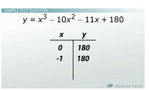
After working out our equation, the y point on the graph will be 180.

First let's solve for x = -1. To do so, we will evaluate our equation by plugging in -1 for all of the x values. Our equation was y = x^3 - 10x^2 - 11x + 180. When we plug in our -1 values for x, it becomes y = (-1)^3 - 10(-1)^2 - 11(-1) + 180. To work this equation, we will need to compute all of the exponents, making our equation y = -1 - 10(1) - 11(-1) + 180. Next, we simply need to multiply our equation, so now we get y = -1 - 10 + 11 + 180. After adding, our solution will be y = 180. So this ordered pair is (-1, 180). We can see that this point on the graph would be beside our y-intercept.

Now we can see that we have two pairs of coordinates in our table: (-1,180) and (0,180). Next, let's evaluate the equation for x = 1. When we let x = 1, we plug in 1 in for all x values. Our equation now looks like y = (1)^3 - 10(1)^2 - 11(1) + 180. We need to solve this equation the same way - by first completing the exponents and then multiplying.

After completing the exponents, our equation looks like y = 1 - 10(1) - 11(1) + 180. Then after multiplying we end up with y = 1 - 10 - 11 + 180. After we add, the solution to this equation will be y = 160. So this ordered pair is (1, 160). By graphing that point, we can see that this point will be to the right of and below our y-intercept.

We now have three pairs of coordinates: (-1, 180), (0, 180) and (1, 160). By knowing these three ordered pairs, we can now check our answer choices to see if we can eliminate either of our remaining choices. At this point, we can see that graph C is not our graph, so the graph that matches the equation would be answer choice D.

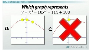
Answer C can be eliminated by knowing what the three pairs of coordinates are.

Sketching for Class

To sketch for a class, you will follow the exact same ideas that we discussed here. The more points that you graph, the better picture you will see of your graph. Oftentimes you will need to plot a couple more points along the graph. If after you've plotted a of couple points and you're still unsure, keep plotting until you're comfortable that you know exactly which graph it will look like.

Lesson Summary

In review, below is a list of steps that will be helpful for you when graphing polynomials:

1. Determine the end behavior of the graph by looking at the lead coefficient.
2. Graph the y-intercept by putting zero (0) in for x values.
3. If you can factor the polynomial, do that; it will be your x-intercepts, but not all polynomials will factor nicely.
4. Remember to graph points where x = -1 and x = 1. These points will help you determine where to plot more points - like in our example (when we decided to plot more points to the right of the origin), in some instances, you will need to plot to the left of the origin.
5. If you are still not sure about the sketch, keep plotting more points. The more points you plot, the more accurate you will be with your answer.